| Home | SPD Curves | Metrics | Proportional | Process SPD | Information |
Further information relating to examination of SPD Curves

What is the Spectral Power Distribution (SPD) of a light?
"In color science and radiometry, a spectral power distribution (SPD) describes the power per unit area per unit wavelength of an illumination (radiant exitance), or more generally, the per-wavelength contribution to any radiometric quantity (radiant energy, radiant flux, radiant intensity, radiance, irradiance, radiant exitance, or radiosity)." Wikipedia
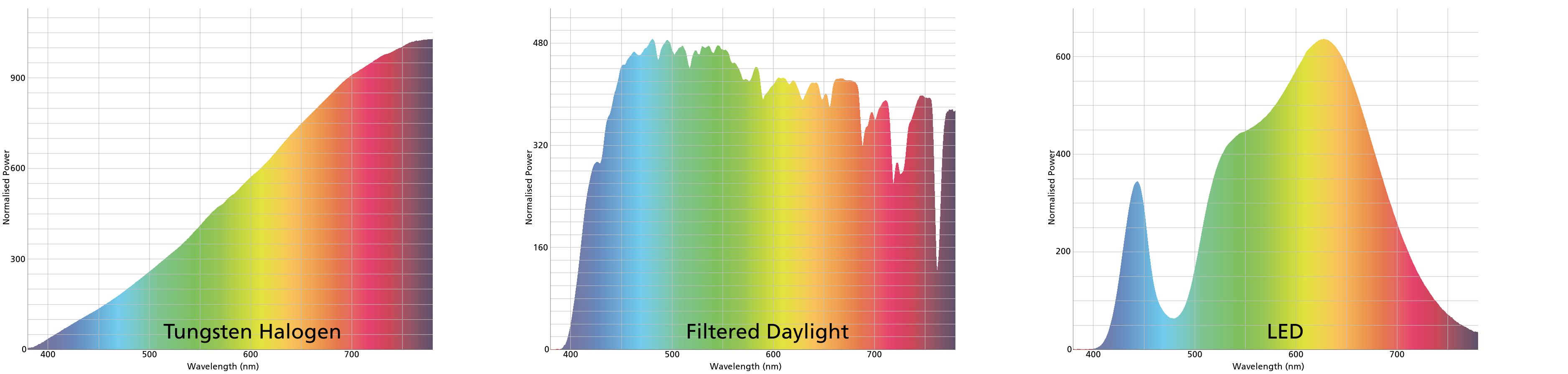 |
Example spectral power distribution (SPD) curves, standard tungsten, filtered daylight and a LED based source. |
In additon to the data presented within this website a number of lower resolution SPD curves of current light source can be seen on the GE Lighting website.
Limitations of only measuring Lux
Lux levels represent a measure of the brightness of a given light as perceived by the human eye, but it does not establish the colour quality of a light, or accurately record the intensity of the light that the human eye is less sensitive to.
When comparing the intensity or power output of a single type of light source, for example tungsten halogen, Lux levels allow for a good comparison of the overall relative light exposure a work of art has been exposed to. However, when many different types of light need to be compared, a similar Lux reading could potentially be produced from a wide range of markedly different SPD curves each representing a different overall relative light exposure.
Recent examinations[1] have shown that differences in the SPD curves of lights at a constant Lux level can effect the rate of fading of some materials, though to a lesser extent than presence or exclusion of UV. So these materials can be seen to have a different sensitivity to light than that of the human eye. Further work may be required to determine how these differences in light sensitivity may alter the long term degradation of materials under different types of light source.
However, it is very easy to measure Lux levels and many museums and galleries already own the required equipment. It would be good if it could still be used as part of a more accurate light level definition. If perhaps new SPD curve specific Lux level limits could be meaningfully recommended for light sensitive work of art.
1: Saunders, David and Kirby, Jo. A comparison of light-induced damage under common museum illuminants. 15th triennial conference, New Delhi, 22-26 September 2008: preprints/ICOM Committee for Conservation. Bridgland, Janet (Editor). ICOM Committee for Conservation (2008), pp. 766-774
Measuring the SPD of a light
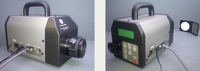
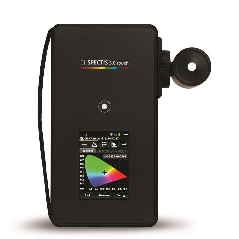
SPD curves are measured using a Spectroradiometer, which are designed to measure the spectral density of an illuminant. They measure the relative intensity of a light source at a number of defined steps across the visible region of the electromagnetic spectrum, generally 380-780nm. Within the National Gallery, London we have used a Konica Minolta CS-1000a Spectroradiometer, to produce 1nm SPD curves. In 2015 an alternative device the GL Optic Spectis Touch 5.0, sensitive from 220-1050nm, was acquired as a replacement. The SPD data can be exported in the form of am XML document and processed, if required, to produces a simple comma separated list of wavelengths and readings, which can be graphed and manipulated within other appropriated pieces of software.
 |
 |
Konica Minolta CS-1000a Spectroradiometer. |
GL Optic Spectis Touch 5.0. |
Light source descriptors
The title/names for each of the light sources presented within this project are constructed in the following way:
| "Supplier or source" "Product code or name of source": "Class of source" - "Published CCT" - "Published CRI" |
| ["Calculated CCT" - "Calculated CRI"] |
| Where the light source class are as follows: |
| LED => Light-emitting diode |
| OLED => Organic light-emitting diode |
| TF => Tungsten Filement |
| TH => Tungsten Halogen |
| FL => Fluorescent lamp |
| CFL => Compact fluorescent lamp |
| MH => Metal halide |
| HPS => High pressure sodium |
| DL => Daylight |
| TS => Theoretical Source |
Normalising SPD based on human perception
As noted before a SPD is the relative spectral output of a given light, measured at a number of defined steps across the visible region of the electromagnetic spectrum. These readings can be expressed in a number of different power related units, which can be graphed to produce a characteristic trace for a given light source. However the actual absolute recorded values are directly proportional to how intense a light source is or even how close it is to the the Spectroradiometer taking the measurements. Therefore in order to compare the SPD curves of different light sources they need to scaled or normalised.
One of the simplest methods is to scale each curve so that either they all have the same maximum value or that they all have the same value at a given wavelength, often at 555nm, which coincides with the peak sensitivity of the human eye.
Lux levels represent a measure of the intensity of a given light as perceived by the human eye. As it is easy to measure the Lux level of a specific light source, scaling SPD curves so they represent the same level of intensity, as perceived by the human eye, allows for a meaningful comparison.
This form of normalisation was carried out as follows:
- Take a SPD data set, scaled between 0 and 1000.
- Multiply the resultant curve by the human photopic sensitivity function, scaled between 0 and 1.
- Calculate the specific total perceived power (Ts) by integrating the area under the resultant curve.
- Calculate a photopic sensitivity scalar (P) using the following function: P = Ta/Ts.
- Where Ta represents an an arbitrary value used to scale the results, here an average total perceived power value was used to ensure that resultant values where still roughly scaled between 0 and 1000. If a specific scale range if not required then just use a Ta value of 1.
- Multiply the value of each point in the original data set by the photopic sensitivity scalar (P) to produce a normalised data set.
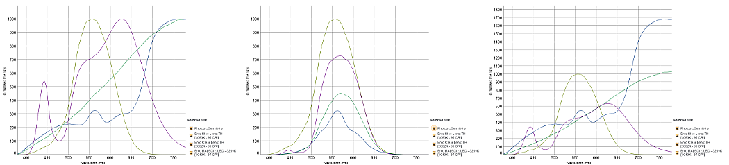 |
Example SPD curves, scaled between 0-1000, multiplied by the photopic sensitivity function and normalised using the appropriate photopic sensitivity scalar. These graphs can be seen more clearly here, here and here |
Relative proportional power distribution
In recent years the use of LED based light sources within museums and galleries have become more common, primarily due to their relatively high efficiency and long life. However, the presence of relatively strong "blue" peaks in their SPD curves have caused some concern among conservation scientists. It has been suggested that this relatively strong peak in the higher energy end of the visible part of the electromagnetic spectrum might increase the rate of light induced fading of sensitive works of art. In fact many of the replacements for standard tungsten halogen lamps contain a substantially higher proportion of "blue" or high energy light. These relative differences can generally be seen by comparing their normalised SPD curves, but it is often clearer to compare the relative intensities of discrete sections of the electromagnetic spectrum rather than the full curve.
In this project the visible range, 380 - 779nm, has been divided into 8 separate 50nm steps; 380 - 429nm, 430 - 479nm, etc. The sum of the power recorded in these separate section could then be displayed in the form of a percentage of the total power recorded over the entire range. To make it easier to compare these sums of power across various different light sources the percentages have actually be calculated relative to the total power recorded over the entire range for a theoretical uniform light source.
In the example below the normalised standard tungsten light source can be seen to have more than twice the total power content measured for one test LED source and the example daylight equivalent (solux) and fluorescent light sources have more than twice the high energy content of the LED source. Each section of the visible spectrum is likely to effect different materials in different ways. As more wavelength dependant fading studies are carried out, the relative importance of these or similar proportional power distributions could help facilitate the choice of appropriate light sources to illuminate particular works of art.
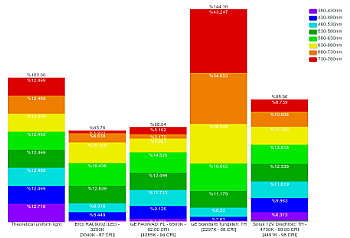 |
Example relative proportional power distribution, the graph can be seen more clearly here. |
Correlated colour temperature (CCT)
"The color temperature of a light source is the temperature of an ideal black-body radiator that radiates light of comparable hue to that light source. The temperature is conventionally stated in units of absolute temperature, kelvin [K]. Color temperature is related to Planck's law and to Wien's displacement law." Wikipedia
The Correlated colour temperature of a light source defines the temperature of the ideal black-body radiator that most closely matches its perceived colour.
The equation required to calculate an approximation of the correlated colour temperature of a given light source is introduced here. The calculation carried out within this particular web site are taken from Version 9.0.1 of the NIST CQS Excel spreadsheet developed by Yoshi Ohno & Wendy Davis, NIST 20/03/2013
Colour rendering index (CRI)
The Colour rendering index of a given light source is a measure of how well it can reproduce the colour of a specific set of test samples relative to an ideal light source with the same colour temperature. Light sources with higher CRI values (95-98) are general recommended for colour critical applications. It should be noted that a high CRI value does not guarantee that a light is capable of reproducing all colours "accurately", only that it will perform as well as a matching ideal light source.
In recent years the CRI value has come under increasing criticism, particularly when it is used to describe light sources with spiky SPD curves, such as fluorescent lamps or white LEDs. A new metric, the Colour quality scale (CQS) is currently under development.
The various equations required to calculate the CRI of a given light source are introduced here and a simplified version of the description with example calculated variables can be seen here.
- Houser K, Mossman M, Smet K, Whitehead L. 2015. Tutorial: Color Rendering and Its Applications in Lighting. Leukos. 12(1,2):7-26. (Free Download)
Colour quality scale (CQS)
The Colour quality scale is new metric being developed to provide a better description of how reliably a given light source can reproduce colour. The CQS values calculated and displayed within this system are calculated using the equation and data included within Version 9.0.1 of the NIST CQS Excel spreadsheet developed by Yoshi Ohno & Wendy Davis, NIST 20/03/2013 and quoted from that spreadsheet:
"This program is shared with you for scientific research exchange purposes only. Please do not use this program directly for your company's products or activities. When you do so, please verify the correctness of the program on your responsibility. NIST is not responsible for any loss to your company caused by any errors in this program.
... CQS is still at research level, and can be used only for your research purposes. It should not be used for your product specification. Note that this version has slightly different CCT factors and scaling factor than those in the SPIE paper. If you publish results from this program, please refer to the papers below:"
TM-30 2015 (2018)
IES TM-30-15 is a standard produced in 2015 to provide a better description of how reliably a given light source can reproduce colour. The TM-30 values calculated and displayed within this system are calculated using the equation and data included within the IES TM-30-15 Excel Basic Calculation Tool, Verion 1.0, released on 21/09/2015.
The current official version of TM-30 is now IES TM-30-18, which can be purchased or downloaded from the IES website at: IES TM-30-18.
The TM-30-15 "... Technical Memorandum describes a method for evaluating light source color rendition that takes an objective and statistical approach, quantifying the fidelity (closeness to a reference) and gamut (increase or decrease in chroma) of a light source. The method also generates a color vector graphic that indicates average hue and chroma shifts, and which helps with interpreting the values of Rf and Rg.
TM-30-15 provides equations and direction for calculating Rf and Rg, including the spectral reflectance functions for the 99 CES. It is accompanied by a software tool to aid in calculation and display of the results (access information for the software tool is provided in the publication). The IES TM-30-15 color rendition method consolidates and synthesizes numerous research efforts that have been ongoing for several years, and was developed by representatives of the manufacturing, specification, and research segments of the lighting industry. ..."
The full Technical Memorandum, IES Method for Evaluating Light Source Color Rendition, can be purchased at: https://www.ies.org, this will also provide access to the Excel based calculation tools."- Specific questions and feedback about the actual TM-30 calculations, beyond the implementation within this website, should be directed to Pat McGillicudyy.
- A. David, P. Fini, K. Houser, Y. Ohno, M. Royer, K. Smet, M. Wei, and L. Whitehead, "Development of the IES method for evaluating the color rendition of light sources," Opt. Express 23, 15888-15906 (2015).
- Further links and discussions related to TM-30 can be found here.
CIE 1976 u'-v' chromaticity distance (Duv)
Duv has been defined as: Closest distance from the Planckian locus on the (u', 2/3 v') diagram, with + sign for above and - sign for below the Planckian locus. (ANSI C78.377-2008) The CIE 1976 u'- v' coordinates of ideal black body radiators follow a curve though the colour space called the Planckian locus, however the coordinates of real light sources, with matching CCTs, will be distributed above and below, positioned along a line perpendicular to the Planckian locus, depending on the quality of the light. The Duv value defines how far the coordinates of a given light are from the ideal position, defined by it's CCT. Calculated Duv values with a magnitude higher than 0.006 are not preferred as a white light and ideally values should have a magnitude of less than 0.001. Further information can be found at here. |
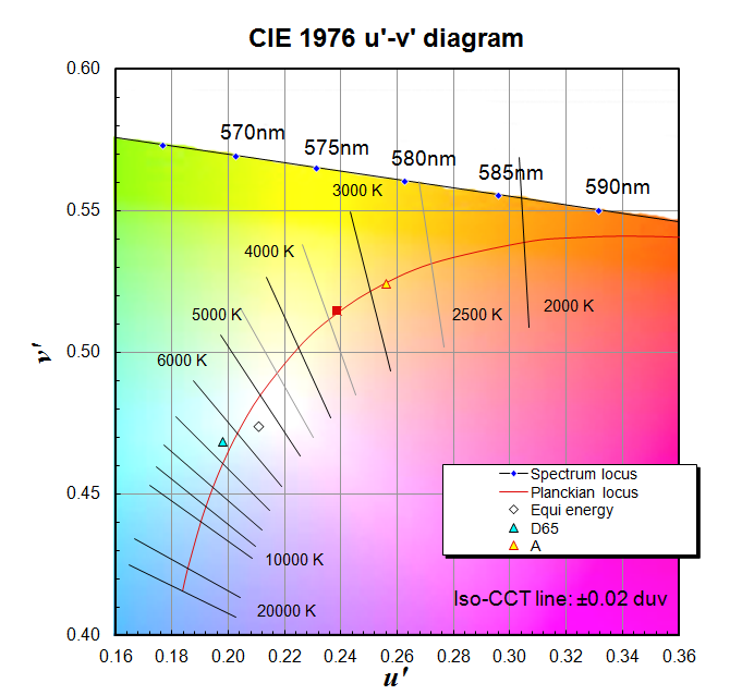 |
Taken from Version 9.0.1 of the NIST CQS Excel spreadsheet developed by Yoshi Ohno & Wendy Davis, NIST 20/03/2013. |
Relative spectral sensitivity: s(λ)dm,rel
The information in this section is mainly based on the work presented in the CIE Technical Collection 1990[2]. The data and functions presented here only represents the average relative spectral sensitivities for museum objects, calculated within the referenced publication. Further object specific relative spectral sensitivity functions could be calculated to demonstrate the specific sensitivities of an individual object.
When it comes to the light induced degradation of museum objects all light is not equal. It is generally accepted that, on average, UV, and to a lesser extent blue light, (with it's lower wavelength and higher energy) can induce more degradation relative to red light (with it's higher wavelength and lower energy) but the exact relationship between wavelength and potential damage, an objects relative spectral sensitivity, is not as widely understood.
By measuring the wavelength dependant degradation of a number of appropriate samples it has been shown[2] that although the exact relative spectral sensitivity for different materials does vary, in general the relationship between wavelength and potential damage can be expressed with the following exponential function:
s(λ)dm,rel = a * exp (-b * λ)[2]
- Where: "a = 1 / exp (-b * 300)"
- and "b" is an average value calculated from measured reference samples.
- In this case a "b" value of 0.012 has been used, which was the value measured for water colours, oil paints on canvas, art paper and textiles.
By examining a graph of this exponential function it can be seen that on average, relative to UV light at 300nm, objects are 0.38 times less sensitive to blue light at 380nm and 0.005 times less sensitive to red light at 740nms
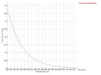 |
The general s(λ)dm,rel function, this graph can be seen in more clearly here. |
2: S. Aydinli, E. Krochmann, G.S. Hilbert, J. Krochmann: On the deterioration of exhibited museum objects by optical radiation, CIE Technical Collection 1990, CIE 089-1991, ISBN 978 3 900734 26 8
Applying s(λ)dm,rel to normalised SPD curves
Applying the general s(λ)dm,rel function was carried out as follows:
- The measured SPD curves are first normalised based on human perception as described above.
- The normalised value at each wavelength point is then multiplied by the appropriate s(λ)dm,rel value.
- The sum of the area under each resultant graph can then be calculated to express the total affective exposure experienced by an object illuminated with a given light source.
- The relative affective exposure can then be calculated for all of the measured light sources by expressing the calculated values as a percentage of the value calculated for a nominated based light source.
- A table of the relative affective exposure values, using a measured daylight SPD curve as the base light source can be seen here.
- Please note at this time these calculation only consider the SPD curves between 380nm and 780nm, if light sources with signals below 380nm are used without UV filtration the numbers calculated will be underestimating the total RE%.
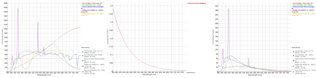 |
Example normalised SPD curves, the s(λ)dm,rel function and the same example SPD curves after the s(λ)dm,rel function has been applied. These graphs can be seen more clearly here, here and here |
Examining how different light source effect the colour of reflected light
When a light is shone on a surface the colour that we perceive is a combination of the SPD curve of the light, the reflectance spectra of the surface and the colour sensitivity of the human eye.
- A measured SPD curve is selected along with the reflectance spectra of a specific surface. The reflectance spectra being the percentage measurement of how much each wavelength of a given light source will be reflected back from a surface.
- By applying each appropriate percentage value to each wavelength value of a specific light source SPD curve the SPD curve of the resultant reflected light can be determined.
- Using the appropriate CIE 1931 colour matching functions this reflected SPD curve can then be transformed into the CIE 1931 XYZ tristimulus values.
- The XYZ value can then be transformed into the CIE Lab colour space, which is commonly used to describe the colour difference.
A page has been constructed to display and compare the CIE Lab value calculated for a each of the 24 patches of a Macbeth ColorChecker under two different light sources and calculate the average CIE ΔE 2000 difference between them. Additional pairs of light sources can be compared by updating the light source selection.
It should be noted that it is not possible to perform a straight conversion from SPD to a coloured patch for some of the patches, under some of the light sources, as their colours cannot be represented within the limited screen RGB colour space without additional mathematical transformation. This represents one of the reasons why it can be difficult to accurately image and reproduce certain colours.
Please also note that at this moment this is a simple representation of converting spectral information into a standard colour space to begin to examine colour gamut issues and colour difference calculations. Further work with colour appearance models, such as CIECAM02, will be required before more accurate theoretical representations of how these colours will appears to the human eye, under different light sources, can be presented.
This page has been set-up to provide more detailed descriptions of the various terms, values and calculations performed to prepare and present the data within this project. Where appropriate links to Wikipedia articles have been provided. For more information about the project in general contact Joseph Padfield.
Measuring and working with different light sources: